Table of Contents

• Introduction
• The Challenge
• The Problem
• Scale / Shape of The Data
• Things that didn’t work
  • Iteration 1: DynamoDB
  • Iteration 2: Elasticsearch
  • Iteration 3: Postgres
• The Data Pipeline
• Evolving The Database Schema
  • Iteration 2: Materialised Columns
  • Iteration 3: Studies Data
  • Iteration 4: Entity, Attribute, Value
• Querying the New Structure (CTEs to the Rescue)
• Iteration 5: Hashing
• Conclusion: Engineering for Scale

I’ve been working on a project at work recently that by my standards has fairly epic scale. While implementing it we’ve had to get deep into the bowels of various databases. This blog post should serve as notes of the things we’ve learned along the way.

TL;DR: Postgres Schemaless Search Journey

We built a high-performance, schemaless search system in Postgres to handle billions of participant records and deliver sub-second queries. Here’s how we did it:

• 🚫 What Didn’t Work: DynamoDB (too slow, expensive), Elasticsearch (blazing reads, but couldn’t keep up with live writes).
• 🛠️ Schema Iterations: Started with JSONB, evolved to promoted columns for top queries, then EAV tables for flexibility.
• ⚙️ Query Optimizations: Used CTEs with WHERE EXISTS to break down complex queries and avoid join explosions.
• 🚀 Performance Fixes: Hashed responses for higher cardinality, partitioned data, and materialized frequent filters.
• 📊 Outcome: Consistent sub-second queries on billions of records.

The Challenge

At its core, my company operates as a marketplace connecting two distinct groups: researchers and participants. Researchers specify detailed requirements for the participants they need for studies, and participants voluntarily provide information that qualifies them for these studies.

A key part of our system is a component we call ‘eligibility,’ which determines which participants meet a researcher’s requirements. While this system has been reliable for years, the platform’s growth—driven by increasing demand for high-quality human data in AI and LLM training—has pushed it to its limits. Scaling this system has been a fascinating technical challenge, and I’ll share what I’ve learned as we’ve worked to address it.

The Problem

The key business requirements of our system are as follows:

• As a researcher, when I’m creating a new study, I want to be able to select the type of participants I need from a series of around 350 pre-defined questions.
  • When I make each selection, I want to be able to see an approximate count of how many participants meet the criteria so that I can see if the participant pool meets my needs. I should be able to do this inside a request response cycle so I can balance the specificity of my requirements with the number of participants that meet them.
• As a researcher, when I publish my study with a given set of requirements I only want my study to be visible / taken by participants that meet those requirements.
• As a participant, when I’m looking for studies to take part in, I want to be able to see a list of studies that I’m eligible for. Again, this should be done inside a request response cycle so I can see the studies that I’m eligible for in a timely manner.

Scale / Shape of The Data

As this challenge is fundamentally a database / search problem I’ll start by outlining the shape of the data we’re dealing with.

• Participant data comes in two forms:
  • ‘question data’ which is essentially a participant’s answers to the 350 pre-defined questions.
    • This data is reasonably slow moving. We might get (on average) one update per participant per day.
    • Questions are added, removed and updated reasonably frequently by another team. This means that we don’t know what the questions or answers will look like in advance, the first we’ll see of a question is a ‘QuestionCreated’ event. Answers can be strings, integers or dates.
  • ‘platform metadata’ which is essentially a record of what the participant has done on our platform. For example if they’ve taken part in a study, or if they’ve been banned.
    • This data is fixed in terms of schema. We only listen to specific events and we know the shape of the events before hand.
    • This data is very fast moving, it’s not uncommon to see millions of events per hour.
    • We need to ingest this data as fast as possible. In business terms, one of the requirements a researcher can place on a study is that participants who take part in study A can’t take part in study B. Both of these studies can be active at the same time.
• In total, we have around 2 million participants and around 1.1 billion pieces of participant data. We can expect to see somewhere in the region of 5000 queries per second at peak times.

In summary, we manage 1.1 billion pieces of participant data for 2 million participants, with peak query rates of 5000/second. Our system must handle dynamic question updates, real-time ingestion of high-velocity events, and ad hoc queries combining arbitrary data points, all while maintaining sub-second response times and excellent write performance.

Things that didn’t work

At this point I’d imagine almost all developers would have a database tool of choice. The good news is I’ve tried a good number of them. Here’s a list of tools we tried and where they fell short:

Iteration 1: DynamoDB

Another of the core requirements for this new system is that it should be explainable. We wanted to be able to answer the question ‘Was Bob eligible for study X on 1st January 2022?’. With this in mind, we opted for our initial ingestion of events to be into an event sourced table in DynamoDB. We built this early on and our first attempt was to read the data back out of the event store to determine eligibility (honestly mostly because it was already there).

DynamoDB is a terrible choice for this problem. Essentially our search algorithm could be boiled down into:

• For each participant, get all events out of the DB and replay them into a participant object.
  • Check if the participant is eligible for the study.

This was slow. Really slow. Our mini test database with 50k participants, each with only around 10 events each took around 35 seconds to query. This would increase quadratically with the number of participants and events. We quickly abandoned this approach.

Note: This would probably have been quicker if we could parallelise the search by participant for example. But this was a non-starter because a) we’re in a lambda environment, so single thread only and b) Dynamo wouldn’t scale and if it did the costs would be insane.

Iteration 2: Elasticsearch

I reckon most people with database experience would scream ‘Elasticsearch’ at this point. And you’d be right. Elasticsearch was actually our tool of choice for part of the existing eligibility system and it performed exceptionally well, returning almost any query in milliseconds.

However, while it was used for count queries in the existing system, it was not used for actually showing participants studies they were eligible for. I never quite understood why, a single source of truth makes loads of sense right? The trouble with ElasticSearch was not the read speed, but the write speed. We needed to be able to ingest millions of events per hour and we needed those events to update the index live. When we started feeding it a live stream of events, the index would quickly become out of date. We tried a few things to mitigate this, but ultimately we couldn’t get it to work.

Iteration 3: Postgres

Postgres is a great general-purpose OLTP database and tends to be the starting point for most projects. Its structured data handling, ACID compliance, and ability to work with JSONB columns made it an appealing candidate for our needs. It seemed like the best of both worlds—a reliable, explainable data store with flexibility for our dynamic requirements.

Ultimately, we settled on Postgres. It provided the right balance of read and write performance, explainability, and schema flexibility. However, scaling Postgres to handle our massive data volume and query requirements came with its own set of challenges. The rest of this article discusses how we tackled those challenges.

The Data Pipeline

The following diagram shows our data pipeline from initial event ingestion through to storing the data in Postgres for querying.

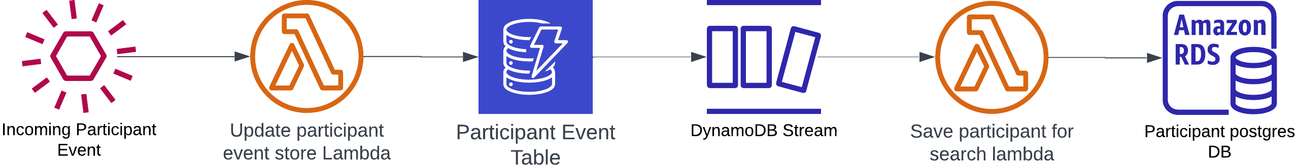
In summary:

• Participant events are ingested and standardised into a format that makes sense to our service.
• We then store these standardised events in the DynamoDB event store.
• The act of saving a new record into DynamoDB triggers a DynamoDB stream…
• Which then triggers a second lambda.
  • There’s a bit of optimisation here, so we don’t hammer Postgres writes, but for simplicities’ sake, we:
  • Get all the data for the given participant back out of DynamoDB and use it to rebuild a complete picture of the participant as they are today.
  • Save the participant to Postgres, overriding the previous version.

Evolving The Database Schema

Firstly, my apologies here. At the time of actually completing this work I was focussed on delivering a product for the business and was moving fast. This means I don’t have great benchmarks for each of the iterations below.

The first iteration of our database schema was incredibly simple. I’ll represent it as typescript here.

1
2
3
4
5
interface Participant {
    id: string,  // uuid
    version: number, // The current version, incremented from the event store.
    data: Record<string, Set<string | number | Date>>
}

Data here is a key-value store where the key is the filter id (a unique identifier assigned to the question) and the value is a set (de-duplicated array) for all the currently valid responses for that filter id. This was a deliberate choice as it allowed us to accommodate question and participant attribute changes without the need for a migration.

So a typical participant might look like:

1
2
3
4
5
6
7
8
9
10
{
  "id": "daveTheLawyer(IYKYK)",
  "version": 110,
  "data": {
    "current-country-of-residence": ["United Kingdom"],
    "first-language": ["English"],
    "studies-started": ["study1", "study2", "study3"]
    // etc....
  }
}

Query Structure

Our queries to this database would come in the form of an Audience, which was a (pretty cool IMO) schema that allowed for the grouping of queries and the logical operations AND, OR and NOT. Here’s a simple example audience for ‘give me all the participants who are left-handed and from Spain’.

1
2
3
4
5
6
7
8
9
10
11
12
13
14
15
16
17
{
  "criteria": {
    "type": "AND",
    "criteria": [
      {
        "type": "SELECT",
        "filterId": "handedness",
        "selectedValues": ["Left"]
      },
      {
        "type": "SELECT",
        "filterId": "current-country-of-residence",
        "selectedValues": ["Spain"]
      }
    ]
  } 
}

But you could get pretty weird with it. Here’s an example where you’re asking ‘Give me all the participants who are EITHER left-handed and from Spain or are between 26 and 35, love pineapple on Pizza and DO NOT know how to juggle.’

1
2
3
4
5
6
7
8
9
10
11
12
13
14
15
16
17
18
19
20
21
22
23
24
25
26
27
28
29
30
31
32
33
34
35
36
37
38
39
40
41
42
43
44
45
{
  "criteria": {
    "type": "OR",
    "criteria": [
      {
        "type": "AND",
        "criteria": [
          {
            "type": "SELECT",
            "filterId": "handedness",
            "selectedValues": ["Left"]
          },
          {
            "type": "SELECT",
            "filterId": "current-country-of-residence",
            "selectedValues": ["Spain"]
          }
        ]
      },
      {
        "type": "AND",
        "criteria": [
          {
            "type": "NUMBER_RANGE",
            "filterId": "age",
            "selectedRange": {"lower": 26, "upper": 35}
          },
          {
            "type": "SELECT",
            "filterId": "favourite-pizza-topping",
            "selectedValues": ["Pineapple"]
          },
          {
            "type": "NOT",
            "criteria": {
              "type": "SELECT",
              "filterId": "juggling-ability",
              "selectedValues": ["Somewhat Proficient", "Proficient", "Expert"]
            }
          }
        ]
      }
    ]
  }
}

Under the hood, we would translate this into an SQL query using an SQL generation script. The simple left-handed Spanish example above would translate into:

1
2
3
4
SELECT *
FROM participants
WHERE data -> 'handedness' ? 'Left'
  AND data -> 'current-country-of-residence' ? 'Spain';

Testing and issues with the first iteration

To test early versions of our database without setting up production infrastructure or importing sensitive participant data, wo wrote a Go script. The script spins up a PostgreSQL database on my modest garage server, populates it with sample data, and runs arbitrary queries for testing.

Issue 1: Querying sub-lists

One of the first issues we encountered was with JSONB array queries, specifically when checking if any items from one array appeared in another JSONB array. There are two possible approaches, one of which was significantly slower.

1
2
SELECT * FROM participants
WHERE data -> 'interests' ?| array['a', 'b'];

While concise, this query performed poorly because it scanned for all possible matches together, which was inefficient.

A faster approach was to split the query into separate checks and combine them with OR, enabling Postgres to optimize the execution plan better:

1
2
3
SELECT * FROM participants
WHERE data -> 'interests' ? 'a'
   OR data -> 'interests' ? 'b';

This approach yielded significantly better performance on large datasets, which is interesting because you achieve exactly the same outcome.

Issue 2: You’re TOAST

To test early database designs without standing up production infrastructure or importing sensitive data, I wrote a Go script to spin up a PostgreSQL database on my garage server, populate it with sample data, and execute arbitrary queries.

The TOAST Problem

We initially tested with 50k participants, each with 100 questions and 100 completed studies. By optimizing query patterns, we reduced most query times to under 2 seconds. We made two incorrect assumptions:

• Performance would scale linearly with more participants and data.
• Upgrading from my eBay micro-PC to a juicy AWS Aurora instance would halve query times.

However, in production, query performance collapsed as participant volume grew. Our investigation revealed two key issues:

1. Real vs. Test Data: Firstly, our actual participant data was not the same shape and size as our test data. We knew it was an approximation but we didn’t know how far away we were. It turns out some participants had completed tens of thousands of studies and answered all the questions. Additionally, after speaking with a team that owned the question and answer data (and events) we moved from a schema which looked like this:

1
2
3
4
5
{
  "type": "SELECT",
  "filterId": "favourite-pizza-topping",
  "selectedValues": ["0"]  // A numeric ID representing the answer index for that question
}

to

1
2
3
4
5
{
  "type": "SELECT",
  "filterId": "favourite-pizza-topping",
  "selectedValues": ["Pineapple"]  // The actual answer text as shown to the participant and researcher.
}

There were good reasons for this, and it seemed like an innocuous change to us at the time (we can match on any string right?) but in some cases the responses are long. Here’s an example::

1
2
3
4
5
{
  "type": "SELECT",
  "filterId": "weekly-exercise",
  "selectedValues": ["I only exercise once per week (such as a single gym class or walking group) outside of my commute to work"]
}

All of this added together meant that in some cases our data field was getting very, very large. When storing large (above 8kb) amounts of data Postgres stores large fields in a TOAST (The Oversized-Attribute Storage Technique) table. This is an internal, compressed side table. Our schema conceptually became:

1
2
3
4
5
6
7
8
9
10
interface Participant { 
    id: string; 
    version: number; 
    dataId: string; 
}

interface ParticipantData { 
    id: string; 
    data: Record<string, Set<string | number | Date>>; 
}

While normal lookups are fast, complex JSONB queries force Postgres to:

• Decompress each TOAST record (which may be split across multiple 8KB pages).
• Execute the query.
• Reverse the foreign key lookup.

This in turn caused our severe performance drop. We’d need to rethink our schema to make this make sense.

Iteration 2

For iteration two, we came up with two new ideas:

Materialised Columns

Fortunately, we had a working system in production from which we could analyze the distribution of filter usage by researchers. As expected, the 80/20 rule applied: 80% of all queries used only 20% of the filters. After discussing with our VP of Data, we adopted a common optimization tactic: materializing frequently used filters by giving them dedicated columns.

We selected the top 10 most-used filters and created dedicated, indexed columns for them. Our schema evolved into:

1
2
3
4
5
6
7
8
interface Participant { 
    id: string; 
    version: number;
    "current-country-of-residence": string[];
    "first-language": string[];
    "etc": string[];
    data: Record<string, Set<string | number | Date>>; 
}

Benefits:

• Queries using only these top filters accessed the indexed columns directly, bypassing the large JSONB column entirely.
• Queries combining promoted filters with others narrowed the participant set before touching the JSONB column, significantly reducing workload

However, the distribution of filter usage could change as time moves on and our users preferences change. Therefore, we decided to:

• Name these columns generically, and map filter-id to column in our application logic.
• Store the ‘promoted’ filters in both the promoted column and the general data area.

This means that if the want to change the ‘promoted’ filters we simply:

• Change the application logic to no longer save filter-id-1 in the promoted column and no longer query for it in the promoted column. Also begin saving filter-id-2 in the promoted column (pull request 1).
• Migrate filter-id-2 data to the promoted column for all participants and start querying for it there (pull request 2).

This approach gave us the best of both worlds: high query performance for common filters and flexibility to adapt as usage patterns evolved.

Splitting The Data Field

We needed to keep the size of the data field as small as possible, to reduce the number of pages per query. However, this was a struggle as new questions would be created arbitrarily and we wouldn’t know the shape of them before we saw the first event, which would look like:

1
2
3
4
5
interface Event {
    type: "ParticipantQuestionAnswered",
    filterId: "testFilter",
    responses: ["some", "responses"]
}

Given this was the only data we had, we decided to split the data field by the first letter of the filter ID, effectively taking one field and turning it into 26. Our schema was now:

1
2
3
4
5
6
7
8
9
10
11
12
13
14
15
16
17
18
19
20
21
22
23
24
25
26
27
28
29
30
31
32
33
34
35
36
37
38
39
40
41
interface Participant {
    id: string;
    version: number;
    promoted_string_column_1: string;
    promoted_string_column_2: string;
    promoted_string_column_3: string;
    promoted_string_column_4: string;
    promoted_string_column_5: string;
    promoted_string_column_6: string;
    promoted_string_column_7: string;
    promoted_string_column_8: string;
    promoted_string_array_column_1: string[];
    promoted_string_array_column_2: string[];
    data_a: Record<string, Set<string | number | Date>>;
    data_b: Record<string, Set<string | number | Date>>;
    data_c: Record<string, Set<string | number | Date>>;
    data_d: Record<string, Set<string | number | Date>>;
    data_e: Record<string, Set<string | number | Date>>;
    data_f: Record<string, Set<string | number | Date>>;
    data_g: Record<string, Set<string | number | Date>>;
    data_h: Record<string, Set<string | number | Date>>;
    data_i: Record<string, Set<string | number | Date>>;
    data_j: Record<string, Set<string | number | Date>>;
    data_k: Record<string, Set<string | number | Date>>;
    data_l: Record<string, Set<string | number | Date>>;
    data_m: Record<string, Set<string | number | Date>>;
    data_n: Record<string, Set<string | number | Date>>;
    data_o: Record<string, Set<string | number | Date>>;
    data_p: Record<string, Set<string | number | Date>>;
    data_q: Record<string, Set<string | number | Date>>;
    data_r: Record<string, Set<string | number | Date>>;
    data_s: Record<string, Set<string | number | Date>>;
    data_t: Record<string, Set<string | number | Date>>;
    data_u: Record<string, Set<string | number | Date>>;
    data_v: Record<string, Set<string | number | Date>>;
    data_w: Record<string, Set<string | number | Date>>;
    data_x: Record<string, Set<string | number | Date>>;
    data_y: Record<string, Set<string | number | Date>>;
    data_z: Record<string, Set<string | number | Date>>;
    data_other: Record<string, Set<string | number | Date>>;
}

N.B. Some of our answers are single select answers and some are multi-select answers. This explains the difference between promoted_string_column_1 and promoted_string_array_column_1.

This has gotten a little more complicated, and our query generator and save functionality got a little more complicated too. Fortunately, our layered architecture meant that we could trap all that complexity in our database layer and our application code was none the wiser.

Benefits:

• Splitting the data by the first letter of the filter id meant we could deterministically save each event without any additional information (such as a map of filterId > table which would need to be kept up to date).
• Splitting the data kept the size of each field small, hopefully small enough to not be too TOASTy.

The results of this were promising. We had reduced the query time again. However, after rebuilding our production database we were still too slow. We’d changed the profile now though, our new database was incredibly quick at querying for the top 10 filter ID’s, but still slow at the long tail of queries.

Iteration 3: Studies Data

Looking at the shape of our production data, we could see that the overwhelming majority of our data was metadata, specifically studies data. This makes sense, as a participant starts and completes far more studies than they answer questions. Unfortunately, it meant that our distribution of data was lop-sided. The data_s column was absolutely massive comparitively to the rest of our data.

Because this type of data was effectively ‘schemad’ (i.e. we knew all participants would have this data, and it wasn’t going to change any time soon.) it made sense to materialise this data too. Postgres can also store arrays! Our schema became:

1
2
3
4
5
6
7
8
9
10
11
12
13
14
15
16
17
18
19
20
21
22
23
24
25
26
27
28
29
30
31
32
33
34
35
36
37
38
39
40
41
42
43
44
45
46
47
48
interface Participant {
    id: string;
    version: number;
    promoted_string_column_1: string;
    promoted_string_column_2: string;
    promoted_string_column_3: string;
    promoted_string_column_4: string;
    promoted_string_column_5: string;
    promoted_string_column_6: string;
    promoted_string_column_7: string;
    promoted_string_column_8: string;
    promoted_string_array_column_1: string[];
    promoted_string_array_column_2: string[];
    studies_started: string[];
    studies_completed: string[];
    studies_approved: string[];
    studies_timed_out: string[];
    studies_returned: string[];
    studies_rejected: string[];
    participant_groups: string[];
    data_a: Record<string, Set<string | number | Date>>;
    data_b: Record<string, Set<string | number | Date>>;
    data_c: Record<string, Set<string | number | Date>>;
    data_d: Record<string, Set<string | number | Date>>;
    data_e: Record<string, Set<string | number | Date>>;
    data_f: Record<string, Set<string | number | Date>>;
    data_g: Record<string, Set<string | number | Date>>;
    data_h: Record<string, Set<string | number | Date>>;
    data_i: Record<string, Set<string | number | Date>>;
    data_j: Record<string, Set<string | number | Date>>;
    data_k: Record<string, Set<string | number | Date>>;
    data_l: Record<string, Set<string | number | Date>>;
    data_m: Record<string, Set<string | number | Date>>;
    data_n: Record<string, Set<string | number | Date>>;
    data_o: Record<string, Set<string | number | Date>>;
    data_p: Record<string, Set<string | number | Date>>;
    data_q: Record<string, Set<string | number | Date>>;
    data_r: Record<string, Set<string | number | Date>>;
    data_s: Record<string, Set<string | number | Date>>;
    data_t: Record<string, Set<string | number | Date>>;
    data_u: Record<string, Set<string | number | Date>>;
    data_v: Record<string, Set<string | number | Date>>;
    data_w: Record<string, Set<string | number | Date>>;
    data_x: Record<string, Set<string | number | Date>>;
    data_y: Record<string, Set<string | number | Date>>;
    data_z: Record<string, Set<string | number | Date>>;
    data_other: Record<string, Set<string | number | Date>>;
}

We rebuilt our production database again, but we were still seeing query latency far higher than we wanted. Our performance profile at this point was:

• Queries for single criteria where the criteria was promoted - Very fast ✅
• Queries for studies data alone - Reasonably fast ⚠️
• Queries for a single non-promoted question - Reasonably fast ⚠️
• Combined queries for promoted data and non promoted data - Slow ❌
• Combined queries for non promoted data - Reaaaally slow ❌

Other notes:

• Query speed dropped as the result set grew. For example, filtering down to 1,200 participants was relatively fast, but querying millions—like all American, English-speaking, car-owning left-handers—was painfully slow. This was because postgres was having to do a lot of searching but not actually eliminating that many records.
• Query time seemed to scale quadratically with the number of filters, rather than linearly. Even then, because some fields were promoted and others weren’t and the number of resulting participants had an effect the performance was literally all over the place.

The overall user experience when you actually plugged this into the app was poor. Slow endpoints are bad, but sort of okay if the performance is consistent. Picture this, you’re a user and you’ve just clicked a new screener in-app. You’ve done this a bunch of times before and you know it takes 20 seconds to return the answer. So you just wait, it’s annoying but tolerable, because you know you’ll get the answer after 20 seconds.

In this case, you’d click one screener and get the answer in 0.8 seconds, then click another and it would take 45 seconds. There was seemingly no pattern to it. Was it broken? Did I do something wrong? It just wasn’t good enough.

At this point I was having a little crisis. Did I make the right choice with Postgres? Could this even be done? Was I going to get the sack for wasting two months faffing around with database schema and producing nothing of value? I decided to spend the weekend really thinking through the idea. We’d learned a bunch of stuff along the way:

• We knew what the shape of our data looked like, including the outliers.
• Postgres can store arbitrary JSONB data and arrays, but don’t ask it to be quick at querying them on large datasets.
• Our system should prioritise a consistent experience on any filter combination over some ultra-fast queries and a long tail of slow ones. If we can’t get every query to be fast the time should at least increase somewhat linearly with query complexity.
• Postgres is very fast at querying lots of records consisting of simple data types where you have indexes which match your query patterns.
• Splitting large datasets into multiple smaller ones, even within the same database, benefits speed greatly.

Iteration 4: Entity, Attribute, Value

N.B. There were a couple more steps in here, but I’m rolling them into one for brevity.

Creating a Schema for ‘schemaless’ data

We needed to be able to store our data as simple datatypes without the need to do migrations whenever new questions were answered. Our solution was to create a table which described the shape of a question rather than a column for each question in the participant table. Our schema would be:

1
2
3
4
5
interface ParticipantResponse {
  participant_id: string
  filter_id: string
  response: string
}

This type of pattern is called an entity-attribute-value table, and is a pretty common pattern.

Key Benefits:

• Really simple data types. Just three strings. We can put a combined index on all of these and search through them very quickly.

Possible Drawbacks:

• Multiple records for one question response. If a participant answers ‘Facebook’ and ‘Instagram’ to the social media question, thats two records.
• We can only store strings. Which means we will have to cast numbers and datetimes in-query to do > or <.

Further Splitting The Data

Additionally, we took the learning from splitting the JSON up and applied it to our new tables. We’d create one of these tables for each letter of the alphabet and store responses according to the first letter of the filter ID.

We also did the same for studies data, but we went a step further and created a table for each of the known filter ids (studies_started, studies_completed etc).

1
2
3
4
5
interface StudiesTable {
  participant_id: string
  // No need for filter id here, the table only contains one type.
  study_id: string
}

Promoting last_active_at

All the count queries had one thing in common. The business requirement for this system was that it should only show matching participants who had been active in the last 90 days. Therefore, it made sense to promote this field into its own column on the participant table.

Resulting Schema

The resulting schema looked a bit mental at first glance, but incorporated everything we’d learned already with these new ideas. We could ingest new questions without the need for a migration and could deterministically query any attribute knowing everything was indexed.

1
2
3
4
5
6
7
8
9
10
11
12
13
14
15
16
17
18
19
20
21
22
23
24
25
26
27
28
29
30
31
32
33
interface ParticipantTable {
    id: string;
    version: number;
    promoted_string_column_1: string;
    promoted_string_column_2: string;
    promoted_string_column_3: string;
    promoted_string_column_4: string;
    promoted_string_column_5: string;
    promoted_string_column_6: string;
    promoted_string_column_7: string;
    promoted_string_column_8: string;
    promoted_string_array_column_1: string[];
    promoted_string_array_column_2: string[];
    last_active_at: Date;
}

interface ParticipantResponseATable {
  participant_id: string
  filter_id: string
  response: string
}
// Repeated through to Z and other (for questions that didn't start with a letter).

interface StudiesStartedTable {
  participant_id: string
  study_id: string
}
// Repeated for studies_completed etc...

interface ParticipantGroupsTable {
  participant_id: string
  participant: string
}

However, this came at the cost of some tricky write logic to parse the homogenous idea of a participant into all these tables and records. There was also some overall data bloat. We were now storing the participant ID n times for each response to each question rather than once.

Querying the new structure (CTE’s to the rescue)

We also introduced a new complexity into the query process. Previously the whole idea of a participant was stored in a single record in a single table, which meant generating a query was relatively easy. However, we now had a single participants data spread across 30+ tables. We needed a way to query across these tables to get the participant ID’s which matched a given set of parameters.

We tried to join the tables when querying but this basically exploded the memory of our postgres instance. After a a few attempts we settled on the use of CTE’s (common table expressions).

CTE’s in postgres are essentially a way to perform a query and create the resulting table in memory. Let’s take an example. We’re looking for left-handed spanish people again. Using a join approach the query would look like:

1
2
3
4
5
6
7
8
9
10
SELECT p.id
FROM participant p
JOIN participant_response_c prc 
  ON p.id = prc.participant_id 
  AND prc.filter_id = 'current-country-of-residence' 
  AND prc.response = 'Spain'
JOIN participant_response_h prh 
  ON p.id = prh.participant_id 
  AND prh.filter_id = 'handedness' 
  AND prh.response = 'left-handed';

This is bad because:

• Join Multiplication (Cartesian Effect): Each participant may have multiple responses (e.g., social media platforms, hobbies). Joining multiple EAV tables without proper filtering creates a huge intermediate result set.
• Lack of Early Filtering: With EAV tables, joining first and filtering later is extremely inefficient because you’re joining large tables on weak keys (participant_id) with many-to-many relationships.
• Inefficient Index Usage: Without proper composite indexes ((participant_id, filter_id, response)), Postgres resorts to slow sequential scans.

The same query refactored to use CTE’s looks like:

1
2
3
4
5
6
7
8
9
10
11
12
13
14
15
16
17
18
19
20
21
22
23
24
WITH country_matches AS (
    SELECT participant_id
    FROM participant_response_c
    WHERE filter_id = 'current-country-of-residence' 
      AND response = 'Spain'
),
handedness_matches AS (
    SELECT participant_id
    FROM participant_response_h
    WHERE filter_id = 'handedness' 
      AND response = 'left-handed'
)
SELECT p.id
FROM participant p
WHERE EXISTS (
    SELECT 1
    FROM country_matches cm
    WHERE cm.participant_id = p.id
)
AND EXISTS (
    SELECT 1
    FROM handedness_matches hm
    WHERE hm.participant_id = p.id
)

When you EXPLAIN ANALYSE this query, it breaks down as follows:

• Perform a simple query where you get all the participant ID’s from participant_response_a where the filter_id is current-country-of-residence and the response is Spain.
• Perform a simple query where you get all the participant ID’s from participant_response_h where the filter_id is handedness and the response is Left.
• Query the base participant table for all participant ID’s which appear in both these tables at least once.

Advantages:

• Each of the sub queries to generate the CTE fully utilises the composite index on (filter_id, response, participant_id), meaning you’re no longer reduced to sequential scans.
• The result of the query is stored in memory as a list of ID’s, the minimum amount of data required to complete the query.
• Each of the CTE queries is parallelisable. Postgres can perform them all in separate worker threads.
• WHERE EXISTS short-circuits the search. If a participant isn’t in the first CTE result set, Postgres never checks the second. This behavior is often faster than a JOIN, which produces large intermediate tables before filtering.
• The addition of the last_active_at filter cut our initial dataset down from 1.8 million participants before we even started to check the CTE’s. By applying the last_active_at filter on the participant table upfront, Postgres performs an index scan on a promoted column, drastically reducing the candidate set for the CTE lookups.
• The creation of each CTE is roughly linear in time, so more filters roughly equals more time. This linear behavior occurs because each CTE runs independently with its own index scan. The final WHERE EXISTS conditions then intersect the results efficiently without compounding complexity.

Outcome

This got us there! The combination of our materialised columns, CTE’s and the last active date meant that we could perform a search on most attributes in under a second on a full database. We were very excited. However, there was still one remaining issue. The query time would still fluctuate depending on the question being asked.

Iteration 5: Hashing

After creating yet another little script to test different combinations of filters we discovered something interesting:

This audience would take under a second:

1
2
3
4
5
6
7
8
9
10
11
12
13
14
15
16
17
{
  "criteria": {
    "type": "AND",
    "criteria": [
      {
        "type": "SELECT",
        "filterId": "handedness",
        "selectedValues": ["Left"]
      },
      {
        "type": "SELECT",
        "filterId": "last-active-at",
        "selectedRange": {"lower": "90 DAYS"}
      }
    ]
  } 
}

But this one would take 18 seconds:

1
2
3
4
5
6
7
8
9
10
11
12
13
14
15
16
17
{
  "criteria": {
    "type": "AND",
    "criteria": [
      {
        "type": "SELECT",
        "filterId": "likes-pineapple-on-pizza",
        "selectedValues": ["Yes"]
      },
      {
        "type": "SELECT",
        "filterId": "last-active-at",
        "selectedRange": {"lower": "90 DAYS"}
      }
    ]
  } 
}

This one was also slow:

1
2
3
4
5
6
7
8
9
10
11
12
13
14
15
16
17
{
  "criteria": {
    "type": "AND",
    "criteria": [
      {
        "type": "SELECT",
        "filterId": "exercise-habits",
        "selectedValues": ["Once per day (for at least an hour) as part of a sports team"]
      },
      {
        "type": "SELECT",
        "filterId": "last-active-at",
        "selectedRange": {"lower": "90 DAYS"}
      }
    ]
  } 
}

Why? Both of these queries look pretty much the same under the hood. After a bit of digging we found that there were two issues at play here.

Indexes and Cardinality

Our data was indexed using the following compound indexes (filter_id, response, participant_id) and (response, filter_id, participant_id). For some reason (which is still unknown to me) Postgres was choosing to use the response index to do the search.

Postgres indexes work better when the cardinality of the index is higher. Given two examples:

• An index with one million records and 100k unique responses.
• An index with one million records and 10k unique responses.

The first index would perform better. This is because postgres can filterv out more records as part of the index scan when the number of unique responses is higher. A lot of our questions have yes / no responses. So by filtering for ‘Yes’ you’d be getting a responses from a large number of filter ids at the same time.

TOAST again

The other problem was that even when whittled down to just the answer, some of the answers were above 8kb, and were still being put into a TOAST table. We needed to slim the response down further.

Solution

Out big realisation here was that we didn’t actually care what the response was, we just needed to match on it. We never need to read the actual response content and display it to the user. This meant that we could hash the response text to create a single, homogenous 32bit response hash.

To solve the cardinality problem, we concatenated the filter ID and the response text into one string before hashing it. This meant that the hashed response for smoker - yes and office based role - yes was different, increasing our cardinality.

Advantages:

• Improved index cardinality for responses with common response text (such as ‘Yes’).
• Consistent response size for all responses, keeping out of the TOAST table.

Disadvantages:

• Even more complex save and query engine, as we now had some data that was hashed and some that was not (studies data).
• Our database was essentially non-human readable. The filter ID’s could be read but the response data was junk.
  • Upside here - some level of data security (though hot much).

Example

Taking our example above:

1
2
3
4
5
6
7
8
9
10
11
12
13
14
15
16
17
{
  "criteria": {
    "type": "AND",
    "criteria": [
      {
        "type": "SELECT",
        "filterId": "exercise-habits",
        "selectedValues": ["Once per day (for at least an hour) as part of a sports team"]
      },
      {
        "type": "SELECT",
        "filterId": "last-active-at",
        "selectedRange": {"lower": "90 DAYS"}
      }
    ]
  } 
}

becomes…

1
2
3
4
5
6
7
8
9
10
11
12
13
14
15
16
17
{
  "criteria": {
    "type": "AND",
    "criteria": [
      {
        "type": "SELECT",
        "filterId": "exercise-habits",
        "selectedValues": ["exercise_habitsOnce per day (for at least an hour) as part of a sports team"]
      },
      {
        "type": "SELECT",
        "filterId": "last-active-at",
        "selectedRange": {"lower": "90 DAYS"}
      }
    ]
  } 
}

becomes

1
2
3
4
5
6
7
8
9
10
11
12
13
14
15
16
17
18
19
20
21
22
23
WITH exercise_matches AS (
    SELECT participant_id
    FROM participant_response_e
    WHERE filter_id = 'exercise-habits'
      AND response = 'HASHED_STRING'
),
last_active_matches AS (
    SELECT id AS participant_id
    FROM participant
    WHERE last_active_at >= NOW() - INTERVAL '90 days'
)
SELECT p.id
FROM participant p
WHERE EXISTS (
    SELECT 1
    FROM exercise_matches em
    WHERE em.participant_id = p.id
)
AND EXISTS (
    SELECT 1
    FROM last_active_matches lam
    WHERE lam.participant_id = p.id
);

Results

This got us where we needed to be! We have since added a few more optimisations to reduce cost and improve latency:

• Added a caching layer to the count endpoint only, where we cache the result for a given query for one hour.
  • From a product standpoint nobody is really fussed if the eligible participant count goes from 18123 to 18129 in an hour. The old system only updated the ES index once per day so this was an improvement.
  • Caching was done by hashing the whole audience (discounting array order etc) so only two requests with the same audience would receive the same result.
  • The actual eligibility ‘calculation’ is done live every time.
• Materialised all none string columns (approval rate, age, joined date etc). Casting a huge amount of strings to ints or dates to do comparisons was costly.

Conclusion: Engineering for Scale: Lessons from Building Schemaless Search in Postgres

This journey of building a schemaless search system in Postgres was far from straightforward. Along the way, we explored different technologies, hit multiple dead ends, and constantly refined our approach based on real-world performance and constraints. Here are some of the biggest lessons we learned:

• Trade-offs are inevitable: No database or pattern solves every problem perfectly. Elasticsearch gave us blazing-fast reads but couldn’t handle our write speed. Postgres gave us control and explainability but demanded careful schema design and indexing.
• Schema evolution is a process, not a decision: Starting with a naive JSONB design worked—until it didn’t. Promoted columns, EAV structures, and hashed responses emerged from iterative improvements and real data insights.
• Performance is about patterns, not just indexes: Query speed depended more on our ability to work with Postgres’ strengths (WHERE EXISTS, CTEs, composite indexes) than simply adding more hardware or caching layers.
• Operational simplicity matters: Postgres let us handle reads and writes without introducing additional infrastructure or synchronization complexity, making our stack simpler to maintain.
• Good enough is good enough: We optimized for consistent, sub-second query times rather than chasing absolute speed on every query. The 80/20 rule (promoted columns for frequent filters) saved us from endless micro-optimizations.

In the end, we achieved our goals: sub-second searches on billions of records and a system flexible enough to handle unpredictable questions without schema changes. It’s not perfect, no system ever is, but it’s fast, scalable, and explainable.

If you’re tackling a similar problem or thinking about scaling Postgres for search, I hope this write-up helps you skip some of the pitfalls we faced.